- 23 Oct, 2023
- read
- Karolinehc
Categories: Digital Marketing SEO Analysis
Tags: SEO Google Search Console CTR Clicks Impressions Numpy Python Average Position Search Analytics
The content presented in this article is intended solely for academic purposes. The opinions expressed are based on my personal understanding and research. It’s important to note that the field of big data and the programming languages discussed, such as Python, R, Power BI, Tableau, and SQL, are dynamic and constantly evolving. This article aims to foster learning, exploration, and discussion within the field rather than provide definitive answers. Reader discretion is advised.
Google Search Console is a free tool provided by Google that helps website owners, webmasters, and SEO professionals monitor and maintain the visibility of their websites in Google’s search results. It provides valuable insights and data about how Google’s search engine crawls and indexes their website.
Let’s begin our analysis with a dataset sourced from Search Console for a venue or event business specializing in weddings. We will also import the necessary libraries from pandas, matplotlib and numpy
import pandas as pd
import matplotlib.pyplot as plt
import numpy as np
SCP = pd.read_csv(r'D:\helen\Documents\PythonScripts\datasets\marketing\SCP2021.csv')
SCP.head()
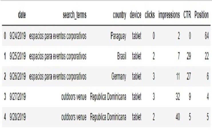
Now, Let’s see the variables, When we call SCP.info(), it will provide us with a summary of the DataFrame, including:
The total number of rows (entries) in the DataFrame. The total number of columns in the DataFrame. The data types of each column. The number of non-null (non-missing) values in each column. The memory usage of the DataFrame.
SCP.info()
SCP.info()
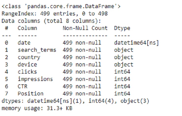
Performance reports in Google Search Console provide valuable data about how our website is performing in Google’s search results. By analyzing metrics like clicks, impressions, click-through rates (CTR), and average position, we can make informed predictions and decisions to improve our website’s visibility and user engagement.
SCP.describe()
Statistics :
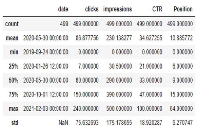
However there isn’t a specific “score” associated with the average position of our pages in search results. Instead, the average position represents the average ranking of our pages for specific search queries. There are several factors influence whether our website’s link is displayed in search results and how often it’s displayed:
Relevance: How well our web page matches the user’s query and intent. Quality: The overall quality of our website’s content and user experience. Ranking: Where our website’s link ranks in the search results for a given query. Search Volume: How often users search for queries related to our content. Competition: How many other websites are competing for the same keywords and queries. So we’ll see in the image a world where only exist five websites and we’ll take the Page Rank as one of the factors to success in google:
Only five websites :
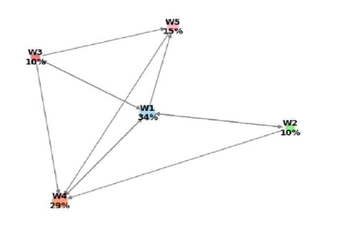
Let’s delve into the PageRank algorithm, which is discussed in detail in the book Pratical Discrete Mathematics by Ryan T. White and Archana Tikayat Ray, 2021, This algorithm, initially developed by students at Stanford University and later adopted by Google founders, assigns weights to web pages based on the importance of their connections. As a result, highly important websites receive higher rankings and appear at the top of search results:
PR(Wj) = (1 - d) / N + d * Σ ( PR(Wi) / C(Wi) )
Where:
PR(Wj): PageRank score for web page Wj.
d: Damping factor, typically set between 0.85 and 0.95.
N: Total number of web pages.
Σ: Summation symbol, indicating a sum over all web pages Wi that link to Wj.
PR(Wi): PageRank score for web page Wi.
C(Wi): Number of outbound links on web page Wi.
PageRank, in essence, employs principles from linear algebra and probability theory to evaluate the significance of web pages based on the number and quality of links pointing to them from other websites.
A = numpy.array([[0, 0.40, 0.40, 0.40, 0.40],
                 [0.5, 0, 0, 0.05, 0],
                 [0.33, 0, 0, 0.10, 0.33],
                 [1, 0, 0, 0, 0],
                 [0, 0, 0, 1, 0]])
The transition probability matrix (A) in the PageRank algorithm represents the likelihood of transitioning from one web page (or node) to another within a network of web pages. Specifically, A[i][j] represents the probability of transitioning from web page i to web page j. In our provided matrix:
#initialize the PageRank vector
v = numpy.array([[0.2], [0.2], [0.2], [0.2], [0.2]])
# the damping factor
d = 0.85
# the size of the "Internet"
N = 5
# compute the update matrix
U = d * A.T + (1 - d) / N
# compute the new PageRank vector
v = numpy.dot(U, v)
# print the new PageRank vector
print(v)
Let’s take the example of A[0][1] = 0.40:
A[0] refers to the first web page, which we can think of as “W1.” A[1] refers to the second web page, which we can think of as “W2.” So, A[0][1] = 0.40 means that there is a 40% chance (or probability) of transitioning from web page “W1” (the first page) to web page “W2” (the second page).
In the context of the PageRank algorithm, this probability is used to simulate how a user might navigate the web by following links on web pages. It’s important to note that this probability matrix is typically constructed based on the structure of the web and the links between pages. The PageRank algorithm then iteratively processes this matrix to compute the importance or PageRank score of each web page.
Here’s what each element of the vector v represents:
v[0]: Represents the initial probability that the user is on web page W1.
v[1]: Represents the initial probability that the user is on web page W2.
v[2]: Represents the initial probability that the user is on web page W3.
v[3]: Represents the initial probability that the user is on web page W4.
v[4]: Represents the initial probability that the user is on web page W5.
In our code, each of these probabilities is set to 0.2, which means that initially, there’s an equal probability of 20% that the user could be on any of the five web pages. This is a simplified starting point for the PageRank calculation.
Output
[[0.3411]
 [0.098 ]
 [0.098 ]
 [0.2935]
 [0.1541]]
So, based on the given PageRank scores:
Website W1 has the highest PageRank score of approximately 34.11%.
Website W4 has the second-highest PageRank score of approximately 29.35%.
Website W5 has the third-highest PageRank score of approximately 15.41%.
Websites W2 and W3 have the lowest PageRank scores of approximately 9.8% each.
So, in terms of ranking position, the order from best to worst is:
W1 W4 W5 W2 and W3 (tied for last place) These rankings are based on the PageRank scores, with higher scores indicating better positions in the search results.
We can conclude that in order to get a high PageRank score, it’s important to create high-quality content for our web page and attract links from other reputable websites.
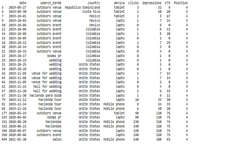
This code will help us display the relevant data from our DataFrame when ‘Position’ equals 4 without truncating any columns.
# Set display options
pd.set_option('display.width', 1000)  # Adjust the width as needed
pd.set_option('display.max_columns', None)  # Display all columns without truncation
better_position = SCP[SCP['Position']==4]
print(better_position)
Relevant data :
High-quality content is more likely to attract the attention of other webmasters and users. When our content is informative, valuable, and relevant to our target audience, other websites are more inclined to link to it as a valuable resource.
Let’s add a new column for the day of the week based on the ‘date’ column.
# Convert the 'date' column to datetime format
SCP['date'] = pd.to_datetime(SCP['date'])

# Create the DataFrame 'SCP_day' from your data
SCP_day = pd.DataFrame(SCP)

# Create a new column for the day of the week
SCP['day_week'] = SCP['date'].dt.day_name()

# Print the DataFrame with the new 'day_of_week' column
print(SCP_day.head())
PageRank, at its core, is a link analysis algorithm. It assigns importance to web pages based on the quantity and quality of inbound links they receive. When authoritative and trusted websites link to our content, it signals to search engines that your content is valuable and trustworthy.
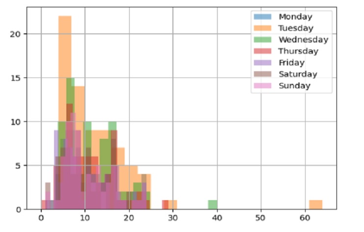
Let’s create a histogram of positions for each day of the week using Matplotlib.
import matplotlib.pyplot as plt

# Create a histogram for each day of the week with a specified label
SCP[SCP['day_week']=='Monday']['Position'].hist(bins = 20, alpha=0.5, label='Monday')
SCP[SCP['day_week']=='Tuesday']['Position'].hist(bins = 20, alpha=0.5, label='Tuesday')
SCP[SCP['day_week']=='Wednesday']['Position'].hist(bins = 20, alpha=0.5, label='Wednesday')
SCP[SCP['day_week']=='Thursday']['Position'].hist(bins = 20, alpha=0.5, label='Thursday')
SCP[SCP['day_week']=='Friday']['Position'].hist(bins = 20, alpha=0.5, label='Friday')
SCP[SCP['day_week']=='Saturday']['Position'].hist(bins = 20, alpha=0.5, label='Saturday')
SCP[SCP['day_week']=='Sunday']['Position'].hist(bins = 20, alpha=0.5, label='Sunday')

# Add a legend
plt.legend()

# Show the plot
plt.show()
Positions for each day of the week :
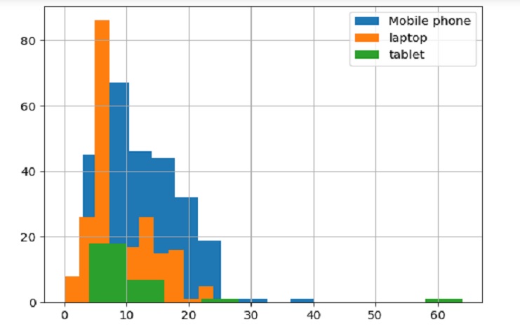
Let’s create a histogram of positions for Different device types (Mobile phone, laptop, and tablet) using Matplotlib.
# Histogram of
SCP[SCP['device']=='Mobile phone']['Position'].hist()

# Histogram of
SCP[SCP['device']=='lapto']['Position'].hist()

# Histogram of
SCP[SCP['device']=='tablet']['Position'].hist()

# Add a legend
plt.legend(['Mobile phone','laptop','tablet'])

# Show the plot
plt.show()
Different device types (Mobile phone, laptop, and tablet) using Matplotlib :
