The content presented in this article is intended solely for academic purposes. The opinions expressed are based on my personal understanding and research. It’s important to note that the field of big data and the programming languages discussed, such as Python, R, Power BI, Tableau, and SQL, are dynamic and constantly evolving. This article aims to foster learning, exploration, and discussion within the field rather than provide definitive answers. Reader discretion is advised.

The exercise displayed here demonstrates the importance of data-driven decision-making in e-commerce and how geographic data and analytics can play a crucial role in targeting consumers effectively. It’s essential to combine data analysis with business strategies to create successful marketing and sales strategies.

Let’s dive into online platforms that host multiple sellers or vendors offering their products or services and discussing sales analytics for a platform where multiple sellers operate.

Let’s import several Python libraries, including pandas, numpy, seaborn, matplotlib, statsmodels, random, geopandas, GeoDatraFrame, and Point from shapely.geometry.

import pandas as pd
import numpy as np
import seaborn as sns
import matplotlib.pyplot as plt
from statsmodels.formula.api import ols
import random
import geopandas as gpd
from geopandas import GeoDataFrame
from shapely.geometry import Point

shop1 = pd.read_csv(r'D:\helen\Documents\PythonScripts\datasets\ecommerce\retail1.csv')
shop2 = pd.read_csv(r'D:\helen\Documents\PythonScripts\datasets\ecommerce\retail2.csv', encoding='iso-8859-1')

Data Cleaning: Ensuring data quality and consistency is essential for making informed decisions. Data cleaning and preprocessing are crucial steps before conducting any analysis.

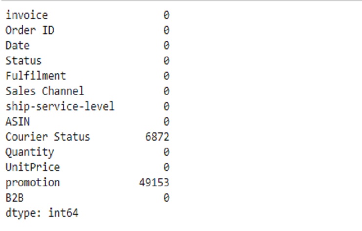
We can see there are missing values

shop1.isnull().sum()
shop2.isnull().sum()

Shop1

Shop2

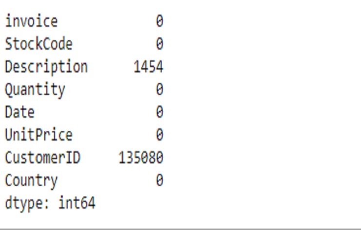
This code effectively removes rows with missing values in the “Description” and “CustomerID” columns and provides us with information on the new shape and the absence of missing values in these columns. It’s a common technique for data preprocessing when dealing with missing data.

# List of columns with missing values
columns_with_missing_values = ["Description", "CustomerID"]

# Drop rows with missing values in the specified columns
shop2 = shop2.dropna(subset=columns_with_missing_values)

# Verify the updated shape and check for missing values again
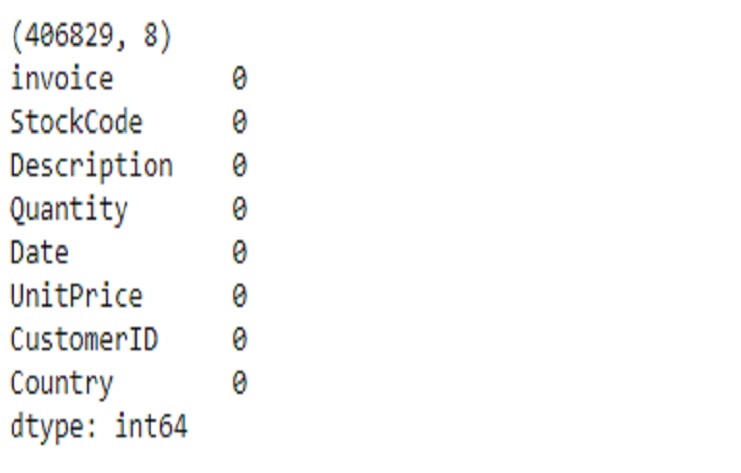
print(shop2.shape)
print(shop2.isnull().sum())

There is no missing values

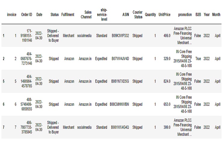
We can use the .head() method to view the first few rows of a DataFrame in pandas, which is a great way to get an overview of the data and its columns.

shop1.head()
shop2.head()

Shop1 dataset

Shop2 dataset

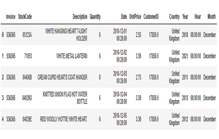
There are 79822 rows and 15 columns for shop1 dataset and 406829 rows and 11 columns for shop2 dataset

We are using the pd.merge() function to merge two DataFrames, shop1 and shop2_final, on multiple columns with an outer join. This means we’re merging the two DataFrames based on the columns specified in on, and it will include all rows from both DataFrames, filling in missing values with NaN where necessary. Then we will use the fillna method to replace the NaN (Not-a-Number) values in our DataFrame with specific values of our choice. The fillna method allows ous to fill in missing or NaN values with another value or a set of values.

shop3 = pd.merge(shop1, shop2_final, on=['invoice', 'Date', 'Quantity', 'UnitPrice', 'Year', 'Month'], how='outer')

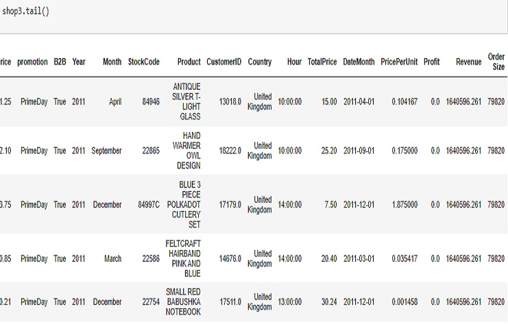
Is useful for quickly inspecting the end of a DataFrame, especially when we want to check the most recent data or verify that our data is correctly loaded and structured.

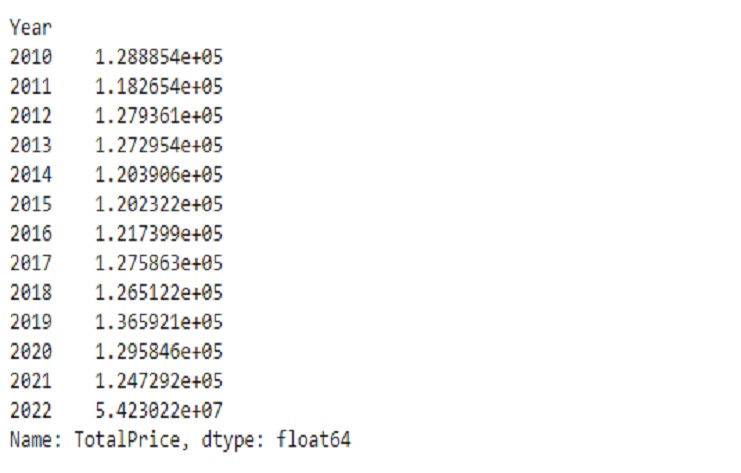
The result is a Pandas Series with the year as the index and the total sales amount as the values for each year. The numbers are expressed in scientific notation because of the default formatting used for large numbers in Pandas. The scientific notation is a way to represent very large or very small numbers in a concise format.

monthly_year = shop3.groupby('Year')['TotalPrice'].sum()
print(monthly_year)

The left column with years (2010, 2011, 2012, etc.) represents the years for which the total sales amount is calculated.

The values: The right column (e.g., 1.288854e+05) represents the total sales amount for each corresponding year. In scientific notation, “e+05” means that the number is multiplied by 10^5, so 1.288854e+05 is equivalent to 128,885.4 (in scientific notation, this is often used for large numbers).

For example, in the output:

In the year 2010, the total sales amount is approximately 128,885.4.

In the year 2011, the total sales amount is approximately 118,265.4.

In the year 2022, the total sales amount is approximately 54,230,220.

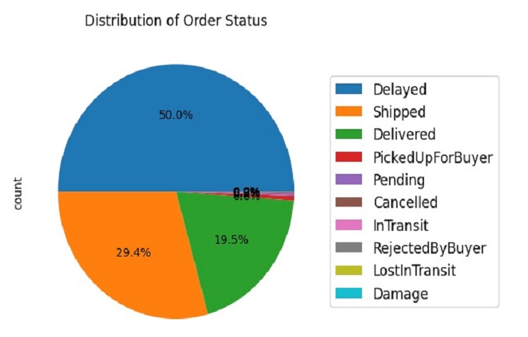
The resulting pie chart will show the distribution of order statuses, and the legend will provide labels for each slice of the pie chart. This visualization helps us understand the proportion of different order statuses in our data.

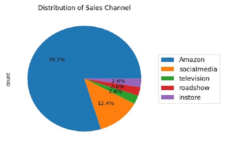
The resulting pie chart will show the distribution of sales channels, and the legend will provide labels for each slice of the pie chart. This visualization helps us understand the proportion of different sales channels in our data.

GroupBy

monthly_year = shop3.groupby('Year')['TotalPrice'].sum()
print(monthly_year)

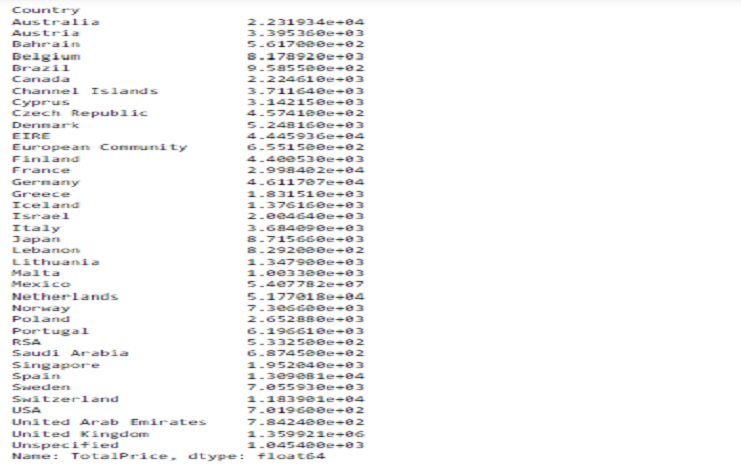
The output will be a Series where the index represents the unique countries in our dataset, and the values represent the total sales for each country. This information can be valuable for analyzing sales performance across different countries in our dataset.

GeoJSON file representing world countries

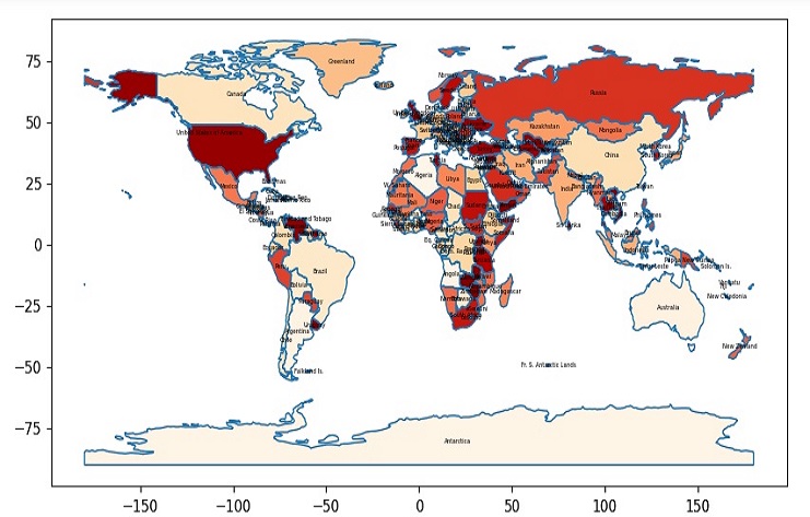
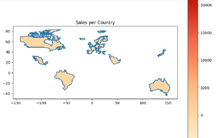
This code will create a map for some countries and display the “TotalPrice” data, using the “OrRd” color map. We can further customize the code to display different information or use a different color map if needed.